Blog
All Blog Posts | Next Post | Previous Post

 Curve Fitting with FNC Math Components
Bookmarks:
Monday, December 27, 2021
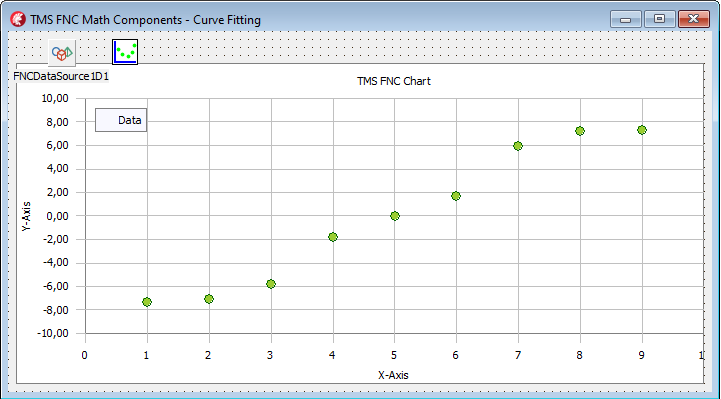
- Discrete data (a series of points) to fit.
- A set of functions (basis functions) to construct the curve.
- A method of solving the fitting problem (optimization algorithm).
- Data (TDataCollection1D) – a collection of points. Each collection item has two properties of real type: ‘V’ – the value of the variable; ‘F’ – the value of the function.
- DataCount (integer) – the number of points in the collection (read-only).
- Data (TFNCDataSource1D) – a data source to show on the chart.
- Chart – a chart to show the data.
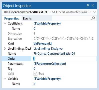
The second ingredient for curve fitting is the set of basis functions. We’ll use the TFNCLinearConstructedBasis1D component. This component provides the easiest way to get a set of functions for constructing the fitted curve. The main published properties of the component are the following
- Variable (TVariableProperty) – provides the name of the variable for the basis functions.
- Coefficient (TVariableProperty) – provides the name of the coefficient for the fitting problem.
- Kind (TBasisKind) – the type of predefined basis functions.
- Order (integer) – number of basis functions for approximation.
- Expression (string) – read-only math expression of the constructed function.
- Parameter (TParameterCollection) – a set of parameter values for parametric basis functions.
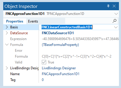
- DataSource (TFNCDataSource1D) – a data source for approximation.
- Basis (TFNCBasis1D) – a basis for approximation.
- Formula (TBaseFormulaProperty) – read-only formula of the curve.
- Expression (string) – read-only math expression of the fitted curve.
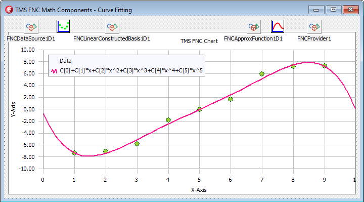
The TFNCApproxFunction1D is a descendant of the TFNCBaseFunction1D component. So, you can draw the curve on an FNC chart as described in the previous article. An example of the resulting curve is shown in the following picture:
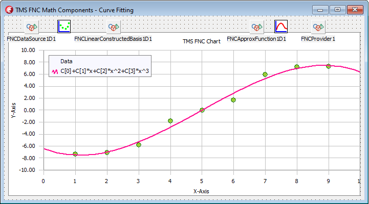
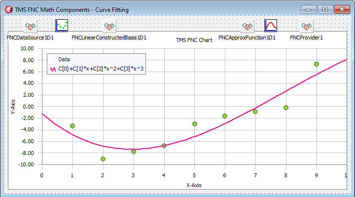
You can change the kind and the order (number of functions) of the basis at design time. Any change leads to the approximation algorithm run, and you can see the resulting curve on the chart. The same is true for the data source: when a point from the collection changed, the curve is reconstructed to fit the new data. In the following two pictures, we showed the approximated curve for the basis Order=6 and for changed data points.
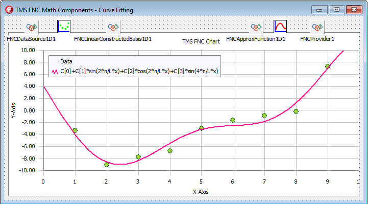
The last option to mention is the Parameters property of the TFNCLinearConstructedBasis1D component. Some basis functions are parametric and they require parameter values for evaluation. For example, the Fourier basis requires the ‘L’ parameter – period of the sine and cosine functions in the Fourier series. When the basis kind changes, the component automatically adds required parameters into the collection, and you can assign the appropriate values to them. An example of the data, approximated with Fourier basis for L=4*Pi is shown in the picture below:
With the FNC math components, you can create the curves fitting application visually, with no line of code. You can tune the components and set the appropriate options at design time to select the best-fitted curve for your data.
The source code of the demo project for the article can be downloaded from here. To start using the FNC math components in your applications you need to install the TMS Analytics & Physics and TMC FNC Chart products.
Bruno Fierens
Bookmarks:

This blog post has not received any comments yet.
All Blog Posts | Next Post | Previous Post